
There is a genre of research note that circulates on trading desks: one page, three charts, a formula box, and a closing line in bold. The good ones compress a career's worth of intuition into something you can pin above a monitor. The bad ones compress a marketing deck.
This post takes one such note — Quant Trading Is Not Prediction: small edges, correct sizing, and repetition are the real business — and does the thing the format cannot do for itself. It rebuilds the claim as a simulation, runs it, and checks whether the numbers on the page are the numbers you actually get.
The headline thesis holds up completely. The supporting arithmetic does not, and the way it fails is more interesting than the thesis.
Everything below is simulated. No live track record is being described, and the point of the exercise is precisely that a plausible-looking track record is weak evidence.
The claim
Stated plainly, the note argues four things:
- Value, not prediction. You do not need to forecast the market. You need positive expected value net of all costs:
EV = E[R] − Costs > 0. - Most of a return is not edge. Decompose the return into market, sector, factor and liquidity components, and what is left over — the residual — is the only part you are actually being paid for.
- Size with discipline. Position sizes follow from the edge and its variance, via Kelly or a fraction of it.
- Repetition does the work. By the law of large numbers, many independent small edges compound into stable performance.
None of that is controversial. What makes the note checkable is that it puts numbers on it: a cumulative return of +24.1% over 10,000 trades, 14.8% annualised, a −9.3% maximum drawdown, a 53.6% win rate, and a Sharpe ratio of 1.27.
Those numbers are the part we can interrogate.
Where the edge actually lives
Start with the decomposition, because it defines what we are even trying to model. On any given day, a book's return is dominated by its exposures — where it happens to be pointed — rather than by any skill in selection.
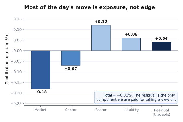
A representative daily decomposition. Market exposure costs 18 bps, sector exposure another 7; factor and liquidity exposures return 12 and 6. The residual — the part attributable to the position selection itself — contributes 4 bps. The book is down 3 bps on the day while the tradable edge was positive.
This is the whole reason the note's title is not a rhetorical flourish. A day on which the strategy did everything right can still be a losing day, because the exposures swamp the residual. If you evaluate the book on its daily P&L you are mostly evaluating its beta. The 4 bps is the business.
Two consequences follow immediately, and both shape the rest of this post. First, the quantity we need to model is the residual return per trade, not the raw return — a number small enough that it will be invisible against daily noise. Second, if the edge is a few basis points and the noise around it is thirty times larger, then distinguishing a real edge from luck is a statistical problem before it is a trading problem.
Modelling one trade
We model a single trade at the position level: what the position returned over its holding period, net of slippage, fees and financing. We want a distribution with three properties the note specifies — a win rate slightly above half, losers slightly larger than winners, and a small positive mean.
Winners are drawn from an exponential distribution with mean W, losers from an exponential with mean L. Exponential tails are the right shape here: most outcomes are small, a few are large, and there is no artificial cap on either side. Given a target mean and standard deviation, W and L are pinned down exactly.
import numpy as np
from scipy.stats import norm

P_WIN   = 0.536      # win rate
MU_T    = 0.0005     # population mean per trade, net of costs (5 bps)
SIGMA_T = 0.0150     # population std per trade (1.5%)


def solve_wl(p, mu, sigma):
    """Exponential win/loss means that match a target mean and std."""
    q = 1.0 - p
    def var_of(W):
        L = (p * W - mu) / q
        return 2.0 * (p * W ** 2 + q * L ** 2) - mu ** 2
    lo, hi = mu / p + 1e-12, 0.20
    for _ in range(200):
        mid = 0.5 * (lo + hi)
        lo, hi = (mid, hi) if var_of(mid) < sigma ** 2 else (lo, mid)
    W = 0.5 * (lo + hi)
    return W, (p * W - mu) / q


W, L = solve_wl(P_WIN, MU_T, SIGMA_T)
b = W / L
print(f"Average winner        {W*100:.4f}%")
print(f"Average loser        -{L*100:.4f}%")
print(f"Payoff ratio b        {b:.4f}")
print(f"Expected value        {(P_WIN*W - (1-P_WIN)*L)*1e4:.2f} bps per trade")
print(f"Kelly fraction f*     {((b*P_WIN - (1-P_WIN))/b)*100:.2f}% of capital")
Output:
Average winner        1.0363%
Average loser        -1.0894%
Payoff ratio b        0.9513
Expected value        5.00 bps per trade
Kelly fraction f*     4.82% of capital
Look carefully at what this strategy is. It wins 53.6% of the time, and when it wins it makes less than it loses when it loses — the payoff ratio is 0.95, below one. There is no asymmetry to point at, no fat right tail, no home runs. The entire edge is that the frequency advantage slightly outweighs the size disadvantage, and it survives costs by five basis points.
Five basis points against a 1.5% standard deviation is a per-trade signal-to-noise ratio of 0.033. That is the honest scale of the thing. Any single trade tells you nothing whatsoever.
The book: twenty-five positions that are not independent
The note's law-of-large-numbers argument requires independent opportunities, and this is where real books diverge from the textbook. We hold 25 positions at a time and turn the book over daily, so 25 trades close each trading day. Those 25 trades are not independent: they are exposed to the same market that day.
We induce that dependence with a one-factor Gaussian copula — a common daily driver that shifts both the probability of winning and the size of the outcome, with an idiosyncratic component on top.
N_CONCURRENT = 25         # positions held at once -> trades closing per day
RHO_LATENT   = 0.25       # loading on the common daily driver
MAG_MIX      = 0.28       # how much of the outcome size loads on that driver
TRADING_DAYS_PER_YEAR = 252

# One fixed affine correction, estimated once on a 10m-trade calibration run,
# so that individual histories keep their own sampling error.
SCALE, SHIFT = 1.1604116477059514, 9.220328770382627e-05


def _raw(rng, n_days):
    W, L = solve_wl(P_WIN, MU_T, SIGMA_T)
    z_day = rng.standard_normal(n_days)[:, None]
    eps = rng.standard_normal((n_days, N_CONCURRENT))
    latent = np.sqrt(RHO_LATENT) * z_day + np.sqrt(1.0 - RHO_LATENT) * eps
    is_win = latent > norm.ppf(1.0 - P_WIN)
    u = rng.random((n_days, N_CONCURRENT))
    u_mixed = np.clip((1 - MAG_MIX) * u + MAG_MIX * norm.cdf(np.abs(latent)),
                      1e-12, 1 - 1e-12)
    mag = -np.log1p(-u_mixed)
    return np.where(is_win, W * mag, -L * mag)


def simulate(n_trades=100_000, seed=20250501):
    """Per-trade position returns, shaped (n_days, N_CONCURRENT)."""
    rng = np.random.default_rng(seed)
    return _raw(rng, n_trades // N_CONCURRENT) * SCALE + SHIFT


r = simulate(100_000)
flat = r.reshape(-1)
corr = (np.corrcoef(r.T).sum() - N_CONCURRENT) / (N_CONCURRENT * (N_CONCURRENT - 1))

print(f"Trades                {flat.size:,}")
print(f"Trading days          {r.shape[0]:,}  ({r.shape[0]/252:.1f} years)")
print(f"Realised mean         {flat.mean()*1e4:.2f} bps per trade")
print(f"Realised std          {flat.std()*100:.2f}%")
print(f"Realised win rate     {(flat>0).mean()*100:.1f}%")
print(f"Avg pairwise corr     {corr:.3f}  (same-day trades)")
Output:
Trades                100,000
Trading days          4,000  (15.9 years)
Realised mean         4.65 bps per trade
Realised std          1.50%
Realised win rate     53.5%
Avg pairwise corr     0.136  (same-day trades)
Note the first discrepancy already. The population edge is 5.00 bps by construction. Over 100,000 trades — sixteen years of daily trading — the realised mean is 4.65 bps. Even at this sample size the estimate is off by 7%.
The average pairwise correlation among same-day trades comes out at 0.136. That is a deliberately modest number, the kind of residual co-movement you get from a reasonably diversified book, and it will turn out to matter enormously.
Repetition: what the law of large numbers actually promises
The note's first panel shows the cumulative average trade return stabilising above zero as repetitions increase, described as "evidence of a persistent edge." The mechanism is real. The timescale is not what the panel implies.
running = np.cumsum(flat) / np.arange(1, flat.size + 1)
for n in (10, 100, 1_000, 10_000, 100_000):
    print(f"after {n:>7,} trades   sample mean = {running[n-1]*1e4:+6.2f} bps")
Output:
after      10 trades   sample mean =  -5.49 bps
after     100 trades   sample mean =  -2.93 bps
after   1,000 trades   sample mean =  -4.40 bps
after  10,000 trades   sample mean =  +2.38 bps
after 100,000 trades   sample mean =  +4.65 bps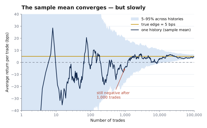
One history's running sample mean (navy) against the true 5 bp edge (gold), with the 5–95% envelope across 120 independent histories in pale blue. Convergence is real but slow: the lower edge of the envelope does not clear zero until around 10,000 trades.
This history has a genuine, positive, permanent 5 bp edge — we put it there — and after a thousand trades it is showing a loss of 4.4 bps per trade. Not a small profit. A loss, on the wrong side of zero. At this book's turnover that is forty trading days; for a slower strategy placing a thousand trades a year, it is a full year of reporting losses on a strategy that is working exactly as designed.
The law of large numbers guarantees convergence. It says nothing about convergence being quick enough to be useful to a trader with a risk committee. The standard error of the mean falls as 1/√n — but our trades are not independent, and the same correlation that will matter for sizing inflates it by √(1 + (n_c − 1)·ρ) = √(1 + 24 × 0.136) = 2.07:
                    independent    with ρ = 0.136    edge / SE
n = 1,000              4.7 bps          9.8 bps         0.51
n = 10,000             1.5 bps          3.1 bps         1.61
n = 100,000           0.47 bps         0.98 bps         5.10
Inverting that to ask how many trades put the edge a given number of standard errors from zero:
edge = 1 × SE   ->    3,838 trades
edge = 2 × SE   ->   15,350 trades
edge = 3 × SE   ->   34,538 trades
So "thousands of times" is the right order of magnitude for the point at which the edge merely equals its own noise — which is not a standard anyone should commit capital against. For a record that would survive a sceptical review, the requirement is tens of thousands. The note's 10,000-trade window lands between one and two standard errors: better than nothing, and nowhere near proof.
Compounding: the part the note gets right
Now size the trades and let them compound. The book allocates 4.30% of capital to each position, which for 25 concurrent positions is a fully-invested book at roughly 1.08× gross exposure. That fraction is chosen to be close to the single-bet Kelly number computed above; we will revisit whether that was wise.
def book_stats(r, f):
    """Equity curve for a book sizing each trade at fraction f of capital."""
    daily = np.log1p(f * r).sum(axis=1)
    equity = 100.0 * np.exp(np.cumsum(daily))
    years = len(daily) / TRADING_DAYS_PER_YEAR
    vol = daily.std(ddof=1) * np.sqrt(TRADING_DAYS_PER_YEAR)
    peak = np.maximum.accumulate(equity)
    return dict(total=equity[-1] / 100.0 - 1.0,
                ann=(equity[-1] / 100.0) ** (1.0 / years) - 1.0,
                vol=vol, sharpe=(daily.mean() * TRADING_DAYS_PER_YEAR) / vol,
                mdd=float((equity / peak - 1.0).min()), equity=equity)


s10k, sall = book_stats(r[:400], 0.043), book_stats(r, 0.043)
print(f"{'':<18}{'first 10,000':>14}{'all 100,000':>14}")
for lbl, k, fmt in [("Total return", "total", "{:+.1%}"),
                    ("Annualised", "ann", "{:.2%}"),
                    ("Volatility", "vol", "{:.2%}"),
                    ("Max drawdown", "mdd", "{:.1%}"),
                    ("Sharpe (ann.)", "sharpe", "{:.2f}")]:
    print(f"{lbl:<18}{fmt.format(s10k[k]):>14}{fmt.format(sall[k]):>14}")
Output:
                    first 10,000   all 100,000
Total return              +10.6%       +622.6%
Annualised                 6.53%        13.27%
Volatility                10.96%        10.55%
Max drawdown              -14.6%        -15.4%
Sharpe (ann.)               0.58          1.18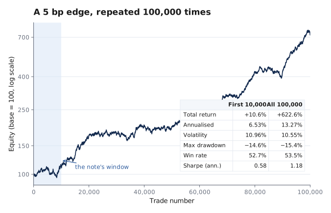
The same 5 bp edge compounded over 100,000 trades at 4.30% of capital per position. The shaded region is the first 10,000 trades — the window the note reports on.
Over the full sample the thesis is vindicated emphatically. A five basis point edge, which is close to nothing, becomes a 13.27% annualised return with a Sharpe of 1.18. Small edges really do compound into meaningful performance. That is the note's central claim and it is correct.
But compare the columns. Over the first 10,000 trades the same strategy returned 10.6% total, 6.53% annualised, with a −14.6% drawdown and a Sharpe of 0.58. The note's figures for a 10,000-trade window were +24.1%, 14.8% annualised, −9.3%, and Sharpe 1.27.
The note has quietly reported the long-run properties of the strategy on a short-run sample. Those are the numbers you converge to after 100,000 trades, not the numbers you should expect to see after 10,000. A fund that raised capital on the strength of the second column and then delivered the first column would have a difficult set of investor conversations, despite the edge being exactly as advertised the entire time.
Sizing, and the correlation trap
The note gives the standard single-bet Kelly formula:
f* = (b·p − q) / b

b = payoff ratio, p = win probability, q = 1 − p
For our strategy that returns 4.82% of capital per bet. The note then says to use a fraction of it, "0.25× in practice," which is sound advice. But the formula is derived for a sequence of independent bets, one at a time. We are placing 25 at once, and they carry an average pairwise correlation of 0.136.
For n concurrent positions with average pairwise correlation ρ, the variance of the aggregate is inflated by a factor of 1 + (n−1)ρ, and the Kelly fraction per position must be deflated by the same factor:
f*_adjusted = f* / (1 + (n − 1)·ρ)
            = 4.82% / (1 + 24 × 0.136)
            = 1.13% per position
The correlation correction is a factor of 4.3. Twenty-five positions with a correlation of 0.136 behave, for sizing purposes, like about six independent ones.
kelly = (b * P_WIN - (1 - P_WIN)) / b
adj = kelly / (1 + (N_CONCURRENT - 1) * corr)

print(f"Single-bet Kelly              {kelly*100:.2f}% per trade")
print(f"Correlation-adjusted Kelly    {adj*100:.2f}% per trade")
print(f"Quarter Kelly (adjusted)      {adj/4*100:.2f}% per trade")
print()
print(f"{'size/trade':>11}{'total':>11}{'annualised':>12}{'max DD':>9}{'Sharpe':>8}")
for f in (adj / 4, adj, 0.043):
    s = book_stats(r, f)
    print(f"{f*100:>10.2f}%{s['total']:>11.1%}{s['ann']:>12.2%}"
          f"{s['mdd']:>9.1%}{s['sharpe']:>8.2f}")
Output:
Single-bet Kelly              4.82% per trade
Correlation-adjusted Kelly    1.13% per trade
Quarter Kelly (adjusted)      0.28% per trade

 size/trade      total  annualised   max DD  Sharpe
      0.28%      14.1%       0.83%    -1.1%    1.19
      1.13%      69.1%       3.36%    -4.3%    1.19
      4.30%     622.6%      13.27%   -15.4%    1.18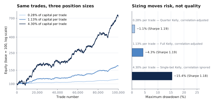
Identical trades, three sizing rules. The Sharpe ratio is unchanged across all three — sizing cannot improve the quality of an edge. What it changes is the scale of the outcome and the depth of the hole you sit in along the way.
Three things are worth taking from this table.
The Sharpe ratio does not move. 1.19, 1.19, 1.18. Position sizing is not a source of edge and cannot manufacture one. It only rescales what the edge produces, in both directions.
The book at 4.30% is running about 3.8× the correlation-adjusted Kelly optimum. This is not conservative sizing that happens to have worked. It is aggressive sizing that happens to have worked in this particular history, and the −15.4% drawdown is the visible symptom. Anyone reading the single-bet Kelly formula off a research note and applying it to a book of concurrent, correlated positions will systematically oversize — and the error compounds with the number of positions, which is exactly the direction people are pushed by "diversify across assets, factors, and time."
Discipline is expensive in the good states. Quarter Kelly turned a sixteen-year, 100,000-trade run of a genuinely profitable strategy into 14.1% total return. That is the honest price of a −1.1% maximum drawdown. The note's framing — "size with discipline" — reads like risk management with no cost attached. It has an enormous cost, and the cost is the entire reason people don't do it.
How much repetition is enough?
The note's weakest link is that it treats 10,000 trades as sufficient repetition. Let us find out what is sufficient, by running the same strategy across 2,000 independent histories at each sample length and asking how often a genuinely profitable strategy shows a losing record.
print(f"{'trades':>8}{'P(losing record)':>19}{'5th pct of mean':>18}")
for n in (250, 500, 1_000, 2_500, 5_000, 10_000, 25_000, 50_000):
    m = np.array([simulate(n, seed=20_000 + s).mean() for s in range(2_000)])
    print(f"{n:>8,}{(m<=0).mean():>18.1%}{np.percentile(m,5)*1e4:>15.2f} bps")
Output:
  trades   P(losing record)   5th pct of mean
     250             38.9%         -28.17 bps
     500             35.4%         -16.96 bps
   1,000             29.7%         -10.96 bps
   2,500             21.6%          -5.72 bps
   5,000             13.2%          -2.26 bps
  10,000              5.8%          -0.10 bps
  25,000              0.4%           1.77 bps
  50,000              0.1%           2.63 bps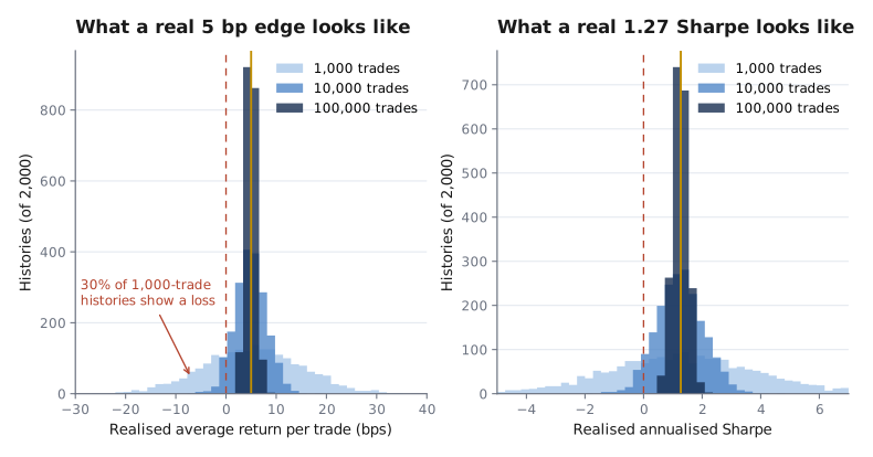
What a genuinely profitable strategy looks like when you only observe part of it. Gold marks the truth (5 bps, Sharpe 1.27); the dashed red line marks zero. At 1,000 trades the realised Sharpe runs from −2.8 to +5.7.
A strategy with a real, permanent, positive edge shows a losing record 29.7% of the time over 1,000 trades. Nearly one in three. At 10,000 trades — the note's window — it still shows a loss 5.8% of the time, and the 5th percentile of realised Sharpe is −0.04.
Read it the other way. A strategy whose true Sharpe ratio is 1.27 produces observed 10,000-trade Sharpe ratios anywhere between −0.04 and 2.57, nine times out of ten. An observed Sharpe inside that window tells you remarkably little about the strategy that produced it.
This is the note's own thesis turned against its own numbers. It says repetition is the real business, and it is right; it then reports a 10,000-trade window as though repetition had done its work, and at 10,000 trades repetition has barely started.
What breaks the edge
The note lists five failure modes. Each of them is a way of destroying a five basis point margin, and having built the simulation we can say how much damage each does.
Overfitting. The 5 bp edge here was assumed into existence. In practice it is estimated from a backtest — and we have just established that a 10,000-trade backtest puts that edge only 1.6 standard errors from zero, which is not a result anyone would accept in another discipline. Every in-sample estimate of a small edge is inflated by selection: you are looking at the strategy precisely because its sample mean was high. If your search produced a 5 bp estimate, the truth is very likely lower.
Data leakage and look-ahead bias. The most dangerous version of this is subtle rather than gross. You do not need a bug that reads tomorrow's close; you need a fill assumption that is optimistic by a fraction of the spread. Half a basis point of unmodelled adverse fill removes 10% of the edge — and against a 1.5% per-trade standard deviation, nothing about the resulting equity curve will look wrong.
Ignoring costs and frictions. The 5 bps here is net. If costs rise by 2 bps, the edge falls to 3 bps — and because the trades needed to establish the edge scale as 1/edge², the sample required to demonstrate it grows by a factor of (5/3)² ≈ 2.8. Rising costs do not just shrink the return, they push verification further out of reach.
Non-stationarity and regime shifts. We assumed a constant edge for sixteen simulated years. No real edge is constant for sixteen years. But note the trap this creates in combination with the previous section: the sample you need to confirm the edge is longer than the period over which the edge can be relied upon to persist. That tension is the central practical problem of systematic trading, and no amount of statistical rigour dissolves it.
Correlation concentration. Already quantified above. An average pairwise correlation of 0.136 — low enough to look like a well-diversified book — costs a factor of 4.3 in the correct position size. The failure mode is not that correlated bets lose money; it is that they justify far less leverage than they appear to, and the discrepancy only becomes visible in the drawdown.
The practical checklist, with the arithmetic attached
The note closes with five checklist items. They are all correct. What they need is the magnitudes.
| Checklist item | What it actually requires here |
|---|---|
| Positive EV after costs | An edge of 5 bps against 150 bps of noise — costs of a few bps are the difference between a business and a hobby |
| Out-of-sample validation | ~35,000 trades to put the edge three standard errors from zero; at 10,000 trades a losing record is a 5.8% event even when the edge is real |
| Correct position sizing | 1.13% per position, not the 4.82% the single-bet Kelly formula gives, because 25 positions at ρ = 0.136 behave like six |
| Many independent opportunities | "Independent" is load-bearing — correlation of 0.136 costs a factor of 4.3 in usable size |
| Live monitoring | Since 10,000 trades cannot confirm the edge, monitoring is not a validation exercise but a decay-detection one |
What the note gets right, and what it gets wrong
The thesis is correct and worth repeating: successful systematic trading is not forecasting. It is finding a margin of a few basis points that survives costs, sizing it so that variance cannot destroy you, and then doing it enough times that the arithmetic asserts itself. The simulation confirms this without qualification. Five basis points, sized at 4.30% of capital per position and repeated 100,000 times, produced a 13.27% annualised return with a Sharpe of 1.18 — from an edge so small that no individual trade could reveal it.
Two things in the note are wrong, and both understate the difficulty:
"Thousands of times" is the floor, not the target. At 10,000 trades the edge sits 1.6 standard errors from zero and the 90% interval on realised Sharpe still touches it. Three standard errors — the sort of margin that survives a sceptical review — takes about 35,000 trades. A note whose central thesis is repetition should not illustrate it with a sample that has not repeated enough.
The Kelly formula on the page is for a bet you are not making. Applied to concurrent, correlated positions it oversizes by a factor equal to 1 + (n−1)ρ, which for any realistic book is not close to one. The formula is right; the note omits the correction that makes it usable, and the omission is in the dangerous direction.
Neither correction damages the argument. If anything they strengthen it. The reason small persistent edges are worth anything is precisely that they are so hard to verify — verification is expensive in a currency, sample size, that cannot be bought. That is the barrier to entry. A strategy whose edge could be established in a thousand trades would have been arbitraged away before you found it.
One trade is noise. Ten thousand trades are still, uncomfortably often, noise. The objective is not to be right about the market; it is to be right by a little, at low cost, with correct sizing — and then to survive long enough for the law of large numbers to finish its work.
This post is for informational purposes only and does not constitute investment advice. All figures are generated from the simulation described above; they are not a track record and past or simulated performance is not indicative of future results.