
Li Zhang, Han Zhang and SuMin Hao, all of the University of International Business and Economics in Beijing, published An equity fund recommendation system by combing transfer learning and the utility function of the prospect theory in The Journal of Finance and Data Science in 2018. It is open access under CC BY-NC-ND, which is why I can reproduce its figures below.
The paper sets itself a real problem. After the 2015 Chinese equity crash, regulators pushed retail participation away from direct stock ownership and toward funds, under an investor appropriateness mandate. That creates a distribution problem: a securities firm has to match a large, sparse, long-tailed population of retail investors to a fund shelf, and most of those investors have no fund transaction history at all. The authors' proposal is to profile investors from their stock trading, where data is plentiful, and carry that profile into the fund market, where it is not.
That instinct is correct. The problem is real, the framing is right, and the cold-start argument holds. What follows is an assessment of whether the execution supports the claims, and it is deliberately unsparing, because this is a paper whose approach I would want to borrow and therefore need to know the failure modes of.
What the system actually does
Strip the terminology and the pipeline is four steps.
Each fund is represented as a vector: nineteen industry allocation weights, a market capitalisation scale coded 5, 3 or 1, an average weekly return over the study window, a return standard deviation, a maximum drawdown, and a largest gain.
Each investor is represented as a vector with a deliberately parallel schema: nineteen industry preference weights derived from their stock purchases, a capitalisation preference on the same 5, 3, 1 coding, an average realised profit rate, a profit standard deviation, a maximum profit rate, and a maximum loss rate.
Candidate generation ranks all funds by inverse Euclidean distance to the investor vector and keeps the top M, with M set to 20.
Re-ranking scores those twenty candidates with a prospect theory value function over three attributes and returns the top N.
The data is 574 equity fund transactions from a single securities branch in Beijing, covering 1 September to 30 December 2015, involving 203 investors and 149 funds. Of those 203 investors, 163 are used to fit parameters and 40 to test.
The transfer learning claim is a naming problem, not a method
The authors are candid about this: they state plainly that they do not add to current methods and only use the concepts of transfer learning. That candour is worth acknowledging, but the label still does real damage to how the contribution should be read.
There is no domain adaptation here. Nothing minimises a discrepancy between a source and target distribution, no shared latent representation is learned, no importance weighting is applied. What actually happens is that a human designed one feature schema and populated it from two different data sources. Industry allocation of a fund and industry preference of an investor are both nineteen-dimensional simplex-ish vectors because the authors chose to define them that way.
This is worth naming precisely, because it is a legitimate and often superior technique. Hand-designed schema alignment is exactly what you should do when the target domain has 574 observations. Any learned adaptation on that sample size would fit noise. The authors made the right engineering decision and then described it with vocabulary that implies a different, more fragile one. A practitioner who reads the abstract and expects transferable machinery will not find any.
The foundational contradiction
Section 3 states that the paper follows the efficient market and rational investment hypothesis of financial theory. Section 5 builds the recommendation score on the Tversky and Kahneman value function.
These are not compatible positions. Prospect theory exists as a direct empirical refutation of rational expected utility maximisation. Its entire content is that people do not evaluate outcomes as rational agents do: they evaluate changes against a reference point, they are concave in gains and convex in losses, and they weight losses roughly twice as heavily as equivalent gains. Adopting its value function while declaring adherence to the rational investment hypothesis is not a synthesis. It is an unresolved contradiction sitting at the base of the model, and it propagates.
The fitted parameters invalidate the mechanism
This is the finding that matters most, and the paper reports it without comment.
The prospect theory value function is defined over the gap between the fund's actual attribute value and the investor's expectation:
V(d) = d^α           for d ≥ 0
V(d) = -θ·(-d)^β     for d < 0
The shape parameters α and β must lie strictly between 0 and 1 for this to be prospect theory. That range is what produces diminishing sensitivity: concave in gains, convex in losses, the characteristic S-curve. The authors know this. They state explicitly that α and β should be smaller than 1, and they initialise at the canonical Tversky and Kahneman values of α = β = 0.88 with loss aversion θ = 2.25.
Their fitting procedure returns α = 1.21 and β = 1.02.
An α of 1.21 is convex in gains. It means the model treats a large positive surprise as more than proportionally better than a small one, which is risk-seeking in the gain domain and the exact opposite of what prospect theory asserts. A β of 1.02 is essentially linear in losses, which removes the convexity that produces the diminishing sensitivity to losses. What survives the fit is the loss aversion coefficient θ = 2.25, and that was never fitted at all. It was fixed at the literature value throughout.
So the component doing the work is a fixed asymmetry multiplier applied to a near-linear function. The paper's stated theoretical contribution, a prospect theory utility function for fund recommendation, is not what the fitted model contains. The improvement over the similarity baseline is real, but it cannot be attributed to prospect theory, because prospect theory's defining shape constraint was violated by the optimiser and the violation was not caught.
Two supporting observations reinforce that the fitting procedure is not to be trusted. The attribute weights are set to (0.3, 0.4, 0.4) "based on our own experience" and never learned; they sum to 1.1 rather than 1. And the search itself is a univariate grid walk in steps of 0.01 that terminates when the change in average accuracy falls below 0.001. That is a stopping rule on a noisy objective computed over 163 investors, not a convergence criterion. It halts where the surface happens to flatten.
An attribute pairing that is almost certainly transposed
Step 4.3 of the algorithm specifies which investor attributes are compared against which fund attributes. As written, the investor triple (average profit rate, maximum profit rate, maximum loss rate) is matched "one by one" against the fund triple (average return, maximum drawdown, largest gain).
Taken literally, that pairs the investor's maximum profit rate against the fund's maximum drawdown, and the investor's maximum loss rate against the fund's largest gain. The sensible pairing is obviously the reverse: profit against gain, loss against drawdown.
This is not pedantry, because the sign of the decision variable follows from it. Under the pairing as printed, the second term is a drawdown minus a positive profit rate, which is negative for essentially every investor and fund pair, and the third term is a positive gain minus a negative loss rate, which is positive for essentially every pair. Two of the three attributes would then contribute a near-constant sign regardless of which investor and which fund are being scored, leaving only the average return term to discriminate. A value function whose inputs are sign-determined by construction is also a plausible mechanical explanation for why the optimiser walked α above 1: it was compensating for structure that carried no information.
I assume this is a typesetting error rather than the implementation. It appears in the operative step of the algorithm, and it is not recoverable from the rest of the text.
The evaluation contains lookahead
The fund attribute vector includes the fund's average weekly return, return standard deviation, maximum drawdown and largest gain, computed over the thirteen weeks from 1 September to 30 December 2015. The investor attribute vector includes realised profit and loss statistics computed over stock trades in that same window. The transactions the recommender is evaluated against also occur in that window.
The system therefore scores each fund using that fund's realised performance over the very period in which the recommendation is notionally being made. At any real decision point, those four numbers do not exist yet.
This is the most consequential problem in the paper for anyone contemplating deployment. It is not a subtle leak through a correlated proxy; the outcome variable is directly in the feature set. The reported accuracy is an upper bound achievable only with hindsight, and the honest version of this experiment requires the fund profile to be computed on a strictly prior window and evaluated on a subsequent one. That experiment is not run, and there is no reason to assume the reported margin survives it.
Reconstructing the paper's own figures
The three figures below are reproduced from the paper.
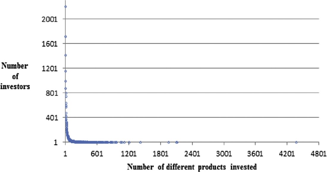
Fig. 1, Distribution of investment products. Reproduced from Zhang, Zhang and Hao (2018) under CC BY-NC-ND 4.0.
Figure 1 makes the sparsity case convincingly. The distribution is severely heavy tailed, which is the paper's justification for abandoning collaborative filtering, and that justification is sound.
Note in passing that the horizontal axis extends to roughly 4365 distinct products for a single investor, while the text describes a universe of "more than 2000 different products". Those two statements cannot both be right. Table 2 carries the same figures, so the inconsistency is in the data description rather than the plot.
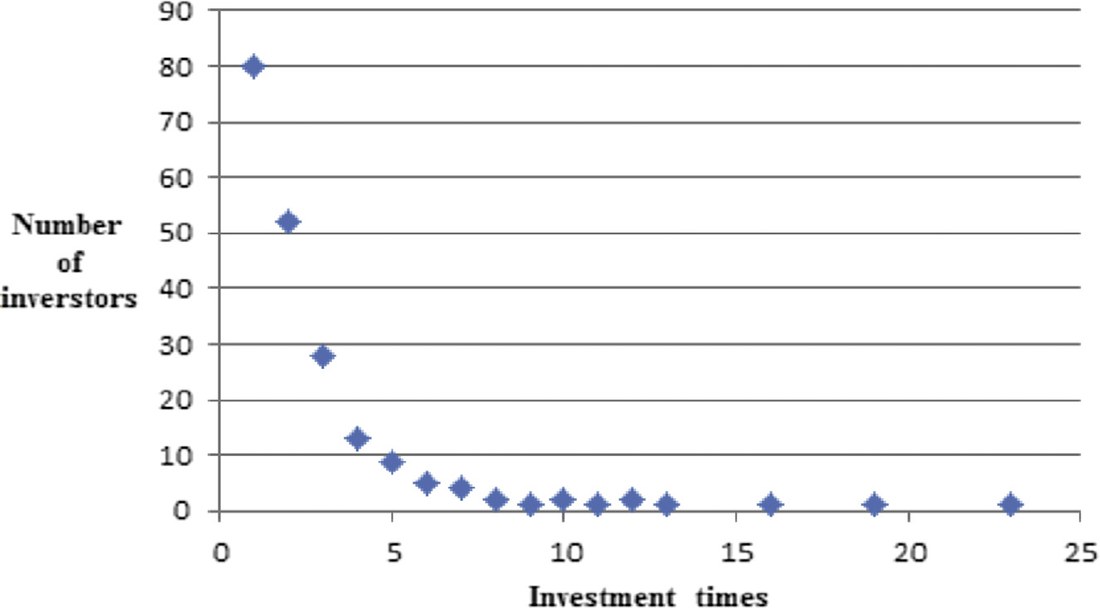
Fig. 2, Distribution of investment occurrences. Reproduced from Zhang, Zhang and Hao (2018) under CC BY-NC-ND 4.0.
Figure 2 is captioned as the distribution of investments per fund, and the body text describes it as the number of investments for each equity fund. It is not. Reading the points off the plot and summing them:
- The vertical values total 203, which is exactly the stated number of fund investors.
- The product of each x value and its y value totals 574, which is exactly the stated number of fund trading records.
Both totals landing precisely on the paper's own sample counts is not coincidence. Figure 2 is the distribution of transactions per investor, not per fund. The caption and the surrounding text are wrong.
This matters, because the paper later justifies its choice of M and N as follows: the mean number of different funds held across the 203 investors is 7.64 and the maximum is 16. Figure 2 says the mean is 574 divided by 203, which is 2.83, and the maximum is 23. Neither number in the text matches the paper's own plot, and 7.64 is not reconcilable with 574 records spread over 203 investors under any reading.
Normalising the results reverses the conclusion
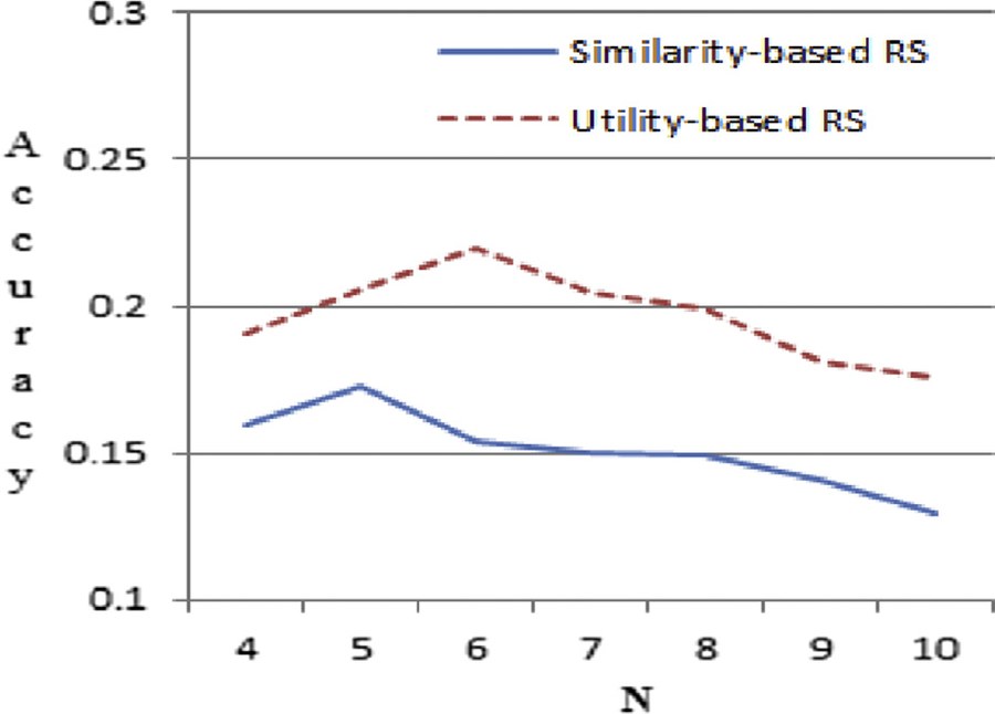
Fig. 3, Recommendation accuracy. Reproduced from Zhang, Zhang and Hao (2018) under CC BY-NC-ND 4.0.
Figure 3 is the headline result. The utility-based system beats the similarity-based system at every N, peaking around 0.22 at N = 6. The authors read this as a sweet spot and note, with appropriate humility, that the accuracy is low compared with the 0.32 achievable in movie recommendation.
That comparison is not meaningful, and neither is the peak, because the metric has a moving ceiling.
The accuracy measure divides the number of correctly recommended funds by N. If an investor bought only two funds and you recommend ten, the best attainable score for that investor is 0.2. As N grows, the maximum possible accuracy falls mechanically. Using the transaction distribution recovered from Figure 2, the ceiling can be computed directly, and the raw scores can be expressed as a percentage of what was actually attainable.
| N | Ceiling | Utility-based | % of ceiling | Similarity-based | % of ceiling |
|---|---|---|---|---|---|
| 4 | 0.542 | 0.191 | 35.2% | 0.160 | 29.5% |
| 5 | 0.463 | 0.205 | 44.3% | 0.173 | 37.4% |
| 6 | 0.403 | 0.220 | 54.6% | 0.154 | 38.2% |
| 7 | 0.357 | 0.207 | 58.0% | 0.150 | 42.0% |
| 8 | 0.320 | 0.199 | 62.3% | 0.149 | 46.6% |
| 9 | 0.290 | 0.183 | 63.2% | 0.140 | 48.4% |
| 10 | 0.265 | 0.177 | 66.8% | 0.130 | 49.1% |
Raw accuracy peaks at N = 6 and declines. Normalised accuracy rises monotonically across the entire range, from 35% to 67%. The apparent optimum at N = 6 is an artifact of the denominator, not a property of the system. The paper's own data says the method gets relatively better as the list gets longer, which is the opposite of what Figure 3 appears to show.
The same normalisation rescues the paper's self-assessment. A raw 0.22 against a ceiling of 0.40 is not a weak result; it is 55% of the attainable maximum. The comparison against 0.32 in movie recommendation is invalid because movie datasets have far denser per-user interaction counts and therefore a far higher ceiling. The authors were harder on themselves than the evidence warranted, for the same reason they misread the shape of their own curve.
Two caveats on my calculation. The ceiling is computed from the full 203-investor distribution, while Figure 3 is measured on the 40-investor test subset, whose distribution may differ. And the accuracy values are read off a published chart, so they carry perhaps half a percentage point of reading error. Neither affects the direction of the result: the ceiling falls by half across the range of N, and no reading error of that size reverses a monotone trend that strong.
The baseline is an ablation
The Similarity-based RS that the method is compared against is not an independent baseline. It is the output of step 4.2 of the same pipeline, truncated at N. So the experiment measures the contribution of the re-ranking stage to the authors' own architecture, which is a useful ablation but does not establish that the architecture beats anything else.
For heavy-tailed transaction data the baseline that matters is popularity: recommend the N most widely held funds to everyone. Figure 1 shows a small number of products drawing enormous investor counts, which is precisely the regime where a popularity baseline is difficult to beat and where personalisation frequently fails to justify itself. That comparison is absent. A random baseline, for reference, would score about 0.019 at any N given 149 funds and 2.83 holdings per investor, so the method is roughly ten times random. That is genuine signal. It is not evidence of personalisation, because popularity would also be far above random.
The strategic error: appropriateness is a constraint, not a similarity score
The paper opens by invoking investor appropriateness, the regulatory principle introduced in response to retail losses in 2015. It then builds a system that ranks funds by proximity between the investor's realised risk and return profile and the fund's realised risk and return profile.
These are different objectives, and the distinction is the whole point of the regulation.
Matching on realised outcomes means an investor who has just taken a 40% maximum loss gets matched to funds exhibiting comparable drawdowns, because that is what minimises the distance. The system reproduces the investor's existing risk exposure and calls it personalisation. It is a model of what this investor has done, which is a reasonable proxy for what they might plausibly buy, and it is being presented as a determination of what they should be sold.
Appropriateness is not a similarity computation. It is a constraint satisfaction problem: establish the investor's risk capacity and tolerance, and exclude products that exceed it, before any ranking occurs. A ranking objective can operate inside that feasible set. It cannot define it. A system that optimises purchase likelihood and is described in the language of suitability is the specific failure mode that appropriateness rules exist to prevent, and the paper does not distinguish the two.
What survives, and what I would do differently
Three things in this paper are worth keeping.
The cold-start framing is correct. Profiling investors in a dense adjacent market and carrying the profile into a sparse one is the right response to 574 observations. Anyone building fund distribution analytics on retail brokerage data faces exactly this shape of problem.
Hand-designed schema alignment beats learned adaptation at this sample size. The authors' actual method, whatever it is called, is the defensible choice. Nineteen industry weights on both sides of the comparison is a sound piece of feature engineering.
Two-stage retrieval then re-rank is the right architecture. Cheap distance-based candidate generation followed by an expensive behavioural scoring function over a short list is standard practice for good reasons, and it is what the paper implements.
Four things I would change before this went anywhere near a production shelf.
Constrain α and β to the unit interval during fitting. If the optimiser wants to leave the valid region, the model is telling you the value function is not the thing driving performance. That is diagnostic information, and it should stop the run rather than be reported as a result.
Rebuild the evaluation on disjoint time windows. Fund attributes from a prior period, transactions from a subsequent one. Until that is done the accuracy numbers describe hindsight, not recommendation.
Report accuracy against its ceiling. Any top-N metric with a variable ceiling should be normalised before anyone reads a shape into the curve. In this paper that single change reverses the conclusion about N.
Separate the appropriateness constraint from the ranking objective, in the architecture. Risk capacity screening first, as a hard filter with its own audit trail. Preference ranking second, inside the surviving set. Conflating them produces a system that is very hard to defend to a regulator and, more to the point, one that recommends the drawdown an investor has already suffered.
The underlying idea is worth developing. The paper does not yet demonstrate that it works.
Zhang L, Zhang H, Hao S. An equity fund recommendation system by combing transfer learning and the utility function of the prospect theory. The Journal of Finance and Data Science, 2018. Published by China Science Publishing & Media Ltd, hosted by Elsevier on behalf of KeAi Communications. Open access under CC BY-NC-ND 4.0. DOI 10.1016/j.jfds.2018.02.003. Supported by the National Social Science Foundation of China, Grant No. 13BTQ027. Figures 1, 2 and 3 are reproduced unaltered under the terms of that licence; the normalisation table is my own calculation from values read off Figures 2 and 3.