Most of what we do as quants is the same small calculation repeated an enormous number of times. We revalue one option along a million Monte Carlo paths. We bump one risk factor and reprice an entire book. We sweep a finite-difference grid for an exotic, node by node, time step by time step. We recalibrate a model by pricing the same instruments thousands of times under slightly different parameters.
The arithmetic in each of these is almost embarrassingly simple. What is hard is the volume. And when the bottleneck is volume rather than logic, we are no longer asking for a faster processor in the everyday sense; we are asking for a machine built to do the same thing to a great many data points at once. That machine is the GPU.
In this article we are going to learn to program it. Not admire it from a distance, not call a black-box library and hope, but actually write the code that runs on the device. We will work in CUDA C/C++, NVIDIA's small set of extensions to ordinary C/C++ that lets us write programs spanning the CPU and the GPU together. The walkthrough follows the classic NVIDIA Introduction to CUDA C/C++ curriculum, but we retell it from the bench of a quantitative researcher, and at every step we ask: where does this show up in our work?
We assume you are comfortable with C or C++. We assume no GPU experience, no parallel-programming experience, and no graphics background. We start, as one should, from "Hello World!".
Why a quant should care about the GPU
To build the right intuition, we have to understand that a CPU and a GPU are optimised for two genuinely different goals.
A CPU is a latency machine. It has a handful of very powerful cores, deep caches, branch prediction, out-of-order execution — an enormous amount of silicon devoted to finishing one sequence of instructions as quickly as possible. If our task is "read this config, parse this trade, decide what to do next," the CPU is exactly right.
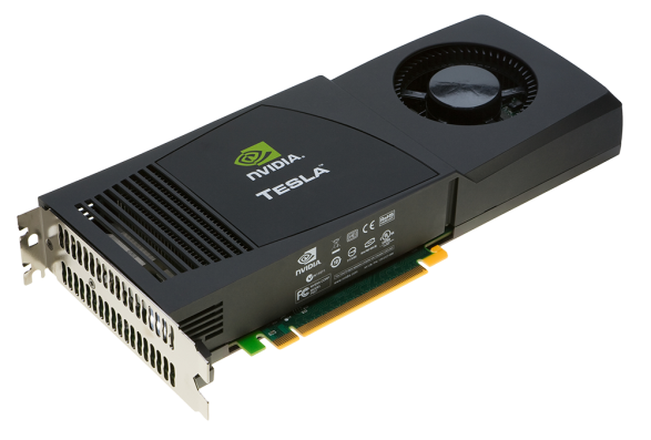
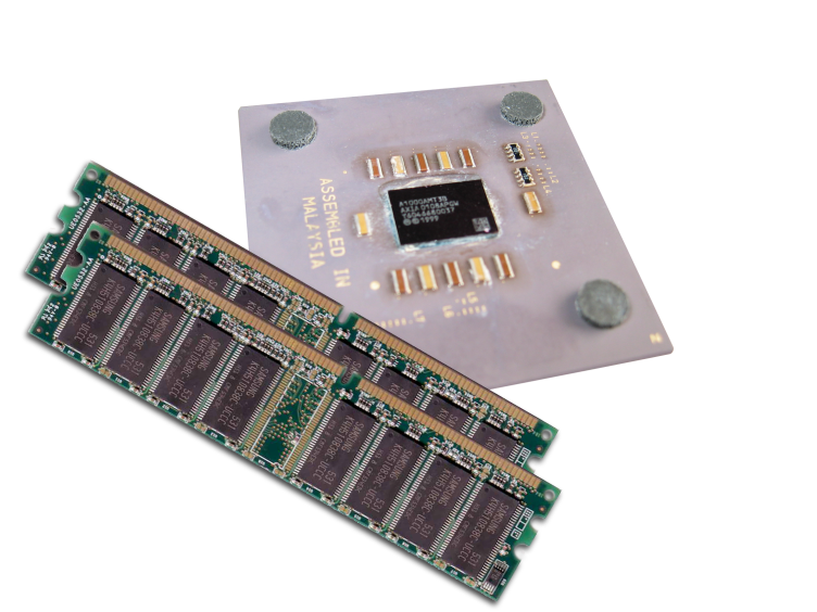
A GPU is a throughput machine. It spends its silicon on many small, simple cores instead of a few clever ones. No single core is impressive; what is impressive is that there are thousands of them, and they can all be doing arithmetic in the same instant. If our task is "apply this identical calculation to ten million independent inputs," the GPU finishes the whole batch in the time the CPU would spend on a small fraction of it.

The same arithmetic, two design philosophies. The CPU pours its transistors into a few sophisticated cores; the GPU spreads them across a sea of simple arithmetic units. A quant's inner loop — one payoff, evaluated across a batch of identical, independent scenarios — is precisely the workload the right-hand machine was built for.
This is why the GPU keeps appearing in our corner of finance: Monte Carlo pricing (millions of independent paths), Greeks by bump-and-revalue (the same pricing function, many times over), historical and Monte Carlo VaR, XVA, finite-difference PDE solvers for exotics, model calibration, and large-scale backtests. The common thread is that we are doing the same arithmetic to a lot of data.
By the end of this article we will be able to:
- Write and launch CUDA C/C++ kernels — functions that run on the GPU;
- Manage GPU memory — move our data to the device and back;
- Manage communication and synchronization between threads — so that cooperating computations get the right answer.
Let us begin with the most important idea of all, the one everything else hangs from.
Heterogeneous computing: host and device
A CUDA program is not a GPU program. It is a program that runs across two processors at once, and the first thing we have to internalise is the vocabulary for that split:
- The host is the CPU and its memory (host memory).
- The device is the GPU and its memory (device memory).
They are separate pieces of hardware, with separate memories, connected over a bus (historically PCI Express). Our data does not magically appear on the GPU; we have to send it there, and we have to bring the results back.
Here is the host — the familiar CPU and its RAM:
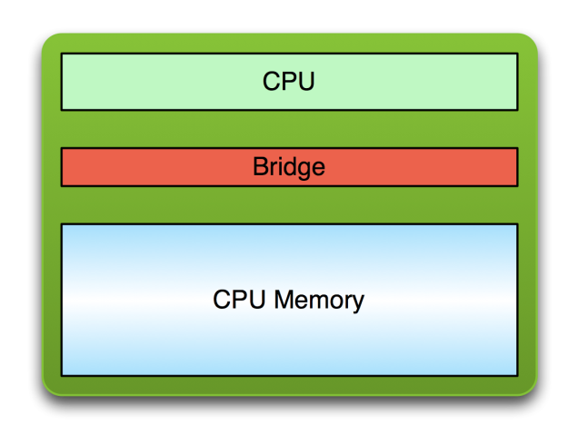
The host is the world we already know: a CPU talking to its own memory through a bridge.
And here is the device — the GPU and its on-board memory:
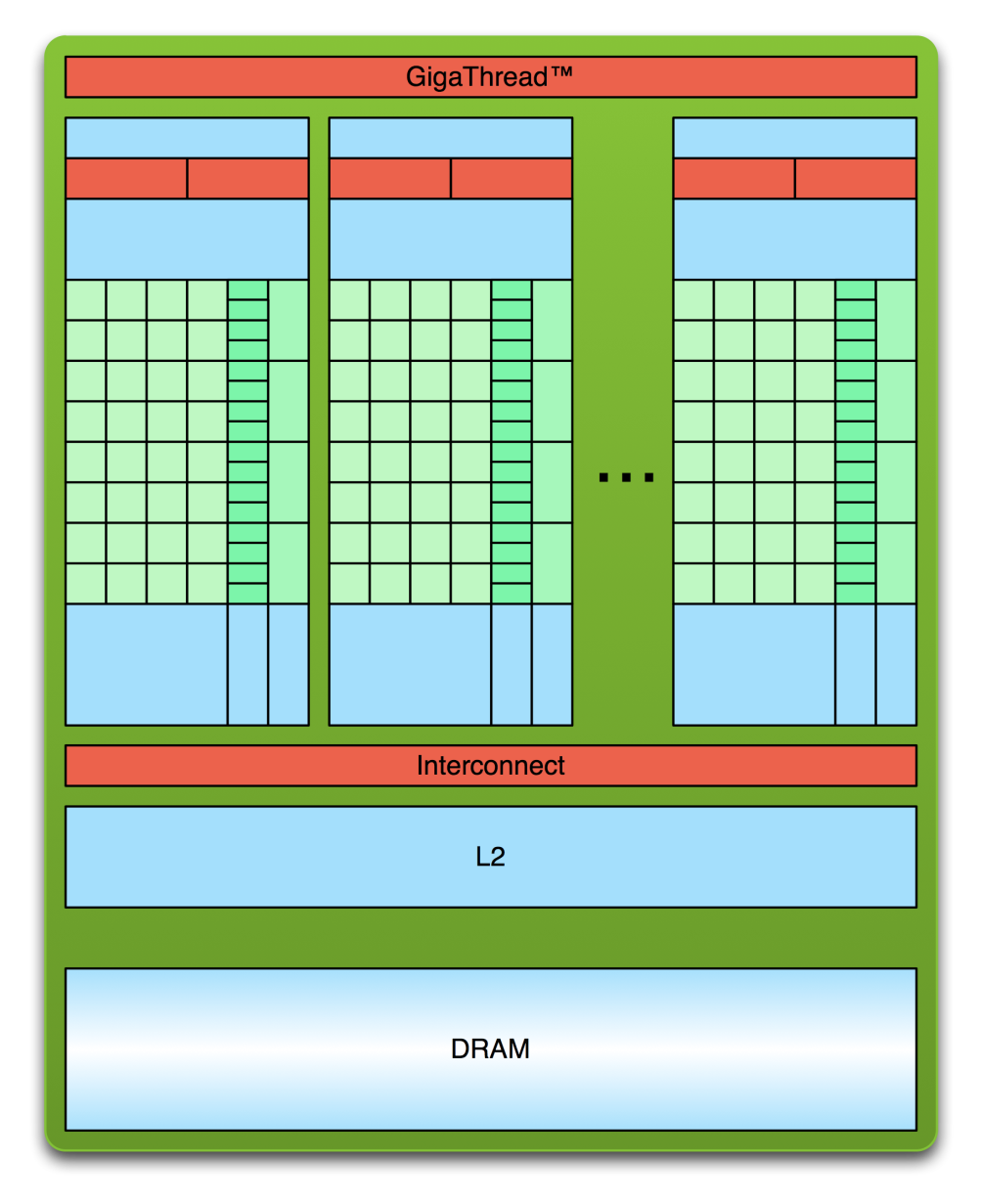
The device is a different animal. A global scheduler feeds work to many independent processing units, each with its own small, fast local memory, all sitting above a shared L2 cache and a large pool of device DRAM. Our job, as we will see, is to keep all of those units busy.
The mental model to carry forward is that a CUDA program is a duet. The host runs the serial orchestration — reading market data, setting up a scenario, deciding what to compute, aggregating the answer. The device runs the hot loop — the massively parallel inner calculation. The art of GPU programming, and certainly of GPU quant programming, is knowing which code belongs where.
A complete program therefore has a recognisable rhythm, which we will see again and again:
- Copy input data from CPU memory to GPU memory.
- Launch the GPU program and execute it, caching data on-chip for performance.
- Copy the results from GPU memory back to CPU memory.
Keep that three-step shape in mind. Every example below is a variation on it.
Hello, GPU: our first kernel
We always start with the program that does nothing useful but proves the toolchain works.
Ordinary C, running entirely on the host, looks like this:
int main(void) {
    printf("Hello World!\n");
    return 0;
}
We compile it with NVIDIA's compiler, nvcc, which is perfectly happy to compile a program that has no device code at all:
$ nvcc hello_world.cu
$ ./a.out
Hello World!
So far there is nothing on the GPU. Let us put something there:
__global__ void mykernel(void) {
}

int main(void) {
    mykernel<<<1, 1>>>();
    printf("Hello World!\n");
    return 0;
}
There are exactly two new syntactic elements here, and they are the heart of CUDA C.
The __global__ keyword. This marks a function that runs on the device but is called from the host. When nvcc sees it, it splits our source file in two: device functions like mykernel() are compiled by NVIDIA's device compiler, and ordinary host functions like main() are handed off to the standard host compiler (gcc, cl.exe, and so on). A __global__ function is called a kernel.
The triple angle brackets <<< >>>. This is a kernel launch: a call from host code into device code. We will return to the two parameters <<<1, 1>>> very shortly — they describe how many parallel copies to run — but the essential point is that this one line is all it takes to execute a function on the GPU.
$ nvcc hello.cu
$ ./a.out
Hello World!
Our mykernel() does nothing, so this is admittedly anticlimactic. But the plumbing is the point: we have compiled a heterogeneous program and launched code on the device. Now we make it compute.
From scalars to vectors: arithmetic on the device
GPU computing is about massive parallelism, so a kernel that does nothing is a poor advertisement. Let us build up from the smallest possible real computation — adding two integers — and grow it into something we would actually run.
Here is a kernel that adds two numbers:
__global__ void add(int *a, int *b, int *c) {
    *c = *a + *b;
}
As before, __global__ tells us add() runs on the device and is called from the host. Notice that the arguments are pointers. Because add() executes on the device, a, b and c must point to device memory. That means we have to allocate memory on the GPU and put our inputs there before we can touch them.
The two memories never mix
This is the rule that trips up everyone exactly once:
- Device pointers point to GPU memory. We may pass them around in host code, but we must not dereference them in host code.
- Host pointers point to CPU memory. We may pass them to device code, but the device must not dereference them.
CUDA gives us a small API for managing device memory that deliberately mirrors the C functions we already know:
| Host C | CUDA device equivalent |
|---|---|
malloc() | cudaMalloc() |
free() | cudaFree() |
memcpy() | cudaMemcpy() |
The full program
Now the host side, main(), in the recognisable copy–compute–copy rhythm:
int main(void) {
    int a, b, c;              // host copies of a, b, c
    int *d_a, *d_b, *d_c;     // device copies of a, b, c
    int size = sizeof(int);

    // Allocate space for device copies
    cudaMalloc((void **)&d_a, size);
    cudaMalloc((void **)&d_b, size);
    cudaMalloc((void **)&d_c, size);

    // Set up input values
    a = 2;
    b = 7;

    // Copy inputs to device
    cudaMemcpy(d_a, &a, size, cudaMemcpyHostToDevice);
    cudaMemcpy(d_b, &b, size, cudaMemcpyHostToDevice);

    // Launch add() kernel on the GPU
    add<<<1, 1>>>(d_a, d_b, d_c);

    // Copy result back to host
    cudaMemcpy(&c, d_c, size, cudaMemcpyDeviceToHost);

    // Cleanup
    cudaFree(d_a); cudaFree(d_b); cudaFree(d_c);
    return 0;
}
The convention of prefixing device pointers with d_ is not required by the language, but it is a discipline worth keeping: in a real pricing engine, mixing up a host and a device pointer is a bug that compiles cleanly and then crashes (or, worse, silently corrupts) at run time.
A quant aside on the data-movement tax. Notice that we spent more lines moving data than computing. Every cudaMemcpy crosses the bus between host and device, and that crossing is slow relative to the GPU's arithmetic. The first rule of GPU performance — and the rule that decides whether a GPU pricer beats its CPU cousin — is move data rarely, compute a lot once it is there. A naive Monte Carlo engine that ships state back and forth every time step will lose to the CPU. A good one copies the inputs up once, does all the work on the device, and copies a small result down at the end.
Running in parallel: blocks
We have run add() exactly once. To use the GPU we want to run it many times at the same time. The change is almost insultingly small:
add<<<1, 1>>>();   // run add() once
add<<<N, 1>>>();   // run add() N times, in parallel
Each parallel invocation of the kernel is called a block. The whole set of blocks is called a grid. Inside the kernel, each block can find out which one it is through the built-in variable blockIdx.x. So if we give every block its own slice of the data, we get vector addition:
__global__ void add(int *a, int *b, int *c) {
    c[blockIdx.x] = a[blockIdx.x] + b[blockIdx.x];
}
By using blockIdx.x to index into the arrays, each block handles a different element, and on the device they run in parallel:
Block 0:   c[0] = a[0] + b[0]
Block 1:   c[1] = a[1] + b[1]
Block 2:   c[2] = a[2] + b[2]
Block 3:   c[3] = a[3] + b[3]
The host code barely changes from before; we just allocate room for N elements and launch N blocks:
#define N 512

// ... cudaMalloc for N*sizeof(int), copy inputs up ...

// Launch add() on the GPU with N blocks
add<<<N, 1>>>(d_a, d_b, d_c);

// ... copy result down, free ...
The quant reading. This toy is more important than it looks. Think of N as the number of Monte Carlo paths, or scenarios, or instruments in a book. Each block handles one. The element-wise pattern — one independent calculation per data point — is exactly how we discount a vector of payoffs, apply a payoff function to a vector of terminal prices, or compute per-path P&L. Vector addition is the "Hello World" of a much larger family of operations we lean on constantly.
Threads
Blocks are not the only way to run in parallel. A block can itself be split into parallel threads. We can rewrite add() to use threads instead of blocks by swapping one built-in variable:
__global__ void add(int *a, int *b, int *c) {
    c[threadIdx.x] = a[threadIdx.x] + b[threadIdx.x];
}
and changing the launch to put the parallelism in the second argument:
// Launch add() on the GPU with N threads (one block)
add<<<1, N>>>(d_a, d_b, d_c);
At this point a reasonable question is: why two different mechanisms for the same thing? Running N blocks of one thread, or one block of N threads, gave the same vector addition. Why bother with threads at all?
The answer — and it is the most important architectural fact in this whole article — is that threads within a block can cooperate, and blocks (cheaply) cannot. Threads in the same block can communicate through a shared scratchpad memory and can synchronize with one another. That is a capability we will need the moment our calculation stops being purely element-wise. Hold that thought; we will cash it in shortly.
Indexing: laying a million paths on the grid
In practice we use both blocks and threads, because that is how the hardware actually schedules work — as a grid of blocks, each containing many threads. That means a single blockIdx.x or threadIdx.x is no longer enough to identify an element. We need a global index, and there is one formula for it that you will type a thousand times:
int index = threadIdx.x + blockIdx.x * blockDim.x;Here blockDim.x is another built-in: the number of threads per block. The picture makes it concrete:

Each block holds blockDim.x threads, numbered locally 0 … blockDim.x − 1. To find an element's position in the global array we offset the local thread index by the blocks that came before it. Here, thread 5 of block 2 (with 8 threads per block) maps to global index 5 + 2 × 8 = 21.
Our combined kernel uses this index directly:
__global__ void add(int *a, int *b, int *c) {
    int index = threadIdx.x + blockIdx.x * blockDim.x;
    c[index] = a[index] + b[index];
}
and we launch enough blocks to cover the data, given a chosen number of threads per block:
#define N (2048 * 2048)
#define THREADS_PER_BLOCK 512

add<<<N / THREADS_PER_BLOCK, THREADS_PER_BLOCK>>>(d_a, d_b, d_c);
When the size is not a round number
Real problems are rarely a friendly multiple of our block size — we do not get to choose 1,048,576 Monte Carlo paths just because it divides nicely. We round the number of blocks up, and then guard against running off the end of the array:
__global__ void add(int *a, int *b, int *c, int n) {
    int index = threadIdx.x + blockIdx.x * blockDim.x;
    if (index < n)
        c[index] = a[index] + b[index];
}add<<<(N + M - 1) / M, M>>>(d_a, d_b, d_c, N);That if (index < n) is not a nicety; it is the difference between a correct kernel and one that reads past the end of device memory. The extra threads in the last block simply do nothing.
The quant reading. This is exactly how we lay a large Monte Carlo run across the device: one path per thread, blockDim.x paths per block, as many blocks as it takes to cover all the paths. The bounds check matters precisely because our path and scenario counts are dictated by accuracy requirements and risk policy, not by what divides our block size.
To summarise what we now have in hand:
- Launch
Nblocks ofMthreads withkernel<<<N, M>>>(...). - Use
blockIdx.xfor the block index,threadIdx.xfor the thread index within the block. - Map data to threads with
int index = threadIdx.x + blockIdx.x * blockDim.x;.
Why threads, really: cooperation, shared memory, and the stencil
So far every element has been independent — thread i reads input i and writes output i, and no thread cares what any other thread is doing. To see why threads exist as a separate level, we need a problem where neighbours talk to each other. The cleanest such problem is the 1-D stencil.
A stencil replaces each element of an array with a weighted combination of its neighbours within some radius. With radius 3, each output element is the sum of the 7 input elements centred on it:

Top: with radius R = 3, every output reads 2R + 1 = 7 inputs. Bottom: a block computes a contiguous tile of outputs but must read a "halo" of R extra inputs on each side — the neighbours that belong to adjacent blocks.
The natural plan is one thread per output element, blockDim.x outputs per block. But look at the cost: with radius 3, each input element is read seven times — once by itself and once by each of its six neighbours' threads. Reading from the device's global memory seven times over is wasteful. This is where thread cooperation finally earns its keep.
Shared memory
Threads within a block can share data through shared memory: a small, extremely fast, on-chip, user-managed scratchpad. We declare it with the __shared__ qualifier, it is allocated per block, and — crucially — it is not visible to threads in other blocks.
The strategy is to cache the tile in shared memory once, then read from the fast scratchpad instead of hammering global memory:
- Read
blockDim.x + 2 × radiusinput elements (the tile plus its two halos) from global memory into shared memory. - Compute
blockDim.xoutput elements from the cached data. - Write
blockDim.xoutputs back to global memory.
Here is the kernel — first attempt:
#define RADIUS     3
#define BLOCK_SIZE 16

__global__ void stencil_1d(int *in, int *out) {
    __shared__ int temp[BLOCK_SIZE + 2 * RADIUS];
    int gindex = threadIdx.x + blockIdx.x * blockDim.x;   // global index
    int lindex = threadIdx.x + RADIUS;                    // local index in temp[]

    // Read this thread's input element into shared memory
    temp[lindex] = in[gindex];

    // The first RADIUS threads also fetch the halos
    if (threadIdx.x < RADIUS) {
        temp[lindex - RADIUS]     = in[gindex - RADIUS];
        temp[lindex + BLOCK_SIZE] = in[gindex + BLOCK_SIZE];
    }

    // Apply the stencil
    int result = 0;
    for (int offset = -RADIUS; offset <= RADIUS; offset++)
        result += temp[lindex + offset];

    // Store the result
    out[gindex] = result;
}
The bug that teaches us synchronization
This kernel is wrong, and the way it is wrong is deeply instructive.
The threads in a block do not all execute in lockstep. Suppose thread 15 races ahead to the result += temp[lindex + offset] loop and reads a halo cell — say temp[19] — before the thread responsible for loading that cell has actually written it. Thread 15 reads stale, uninitialised memory. The answer is silently wrong. This is a data race, and on a GPU, with thousands of threads in flight, races are the rule, not the exception.
The fix is a barrier:
void __syncthreads();__syncthreads() synchronizes all threads within a block: every thread must reach the barrier before any thread is allowed past it. We use it to separate the "load the shared tile" phase from the "use the shared tile" phase, which prevents the read-after-write, write-after-read, and write-after-write hazards (RAW / WAR / WAW) that data races create. One caveat the hardware imposes: if __syncthreads() sits inside conditional code, the condition must be uniform across the block — every thread must take the same branch to the barrier, or some threads will wait forever.
The corrected kernel simply inserts the barrier between loading and computing:
__global__ void stencil_1d(int *in, int *out) {
    __shared__ int temp[BLOCK_SIZE + 2 * RADIUS];
    int gindex = threadIdx.x + blockIdx.x * blockDim.x;
    int lindex = threadIdx.x + RADIUS;

    // Read input elements into shared memory
    temp[lindex] = in[gindex];
    if (threadIdx.x < RADIUS) {
        temp[lindex - RADIUS]     = in[gindex - RADIUS];
        temp[lindex + BLOCK_SIZE] = in[gindex + BLOCK_SIZE];
    }

    // Synchronize: ensure all the data is in shared memory before we read it
    __syncthreads();

    // Apply the stencil
    int result = 0;
    for (int offset = -RADIUS; offset <= RADIUS; offset++)
        result += temp[lindex + offset];

    out[gindex] = result;
}
To recap the cooperation toolkit:
- Use
__shared__to declare a variable or array in shared memory. The data is shared between threads of a block and invisible to other blocks. - Use
__syncthreads()as a barrier to prevent data hazards.
The punchline for quants: a stencil is a finite-difference PDE step
Here is where the toy stops being a toy. That stencil — each new value is a weighted sum of neighbouring old values — is exactly the shape of an explicit finite-difference scheme for a partial differential equation. And PDEs are how we price a great many derivatives.
Recall the Black–Scholes PDE for the value V(S, t) of an option:
∂V/∂t + ½ σ² S² ∂²V/∂S² + r S ∂V/∂S − r V = 0To solve it numerically we lay down a grid in asset price S and in time t, and we approximate the derivatives with differences between neighbouring grid nodes. The explicit scheme then expresses the value at node i at the next time level n+1 purely in terms of three neighbouring nodes at the current level n:
V[i, n+1] = α·V[i-1, n] + β·V[i, n] + γ·V[i+1, n]
One explicit time step: the new value at node i is a weighted sum of three old neighbours. The coefficients α, β, γ come from the discretised PDE; for Black–Scholes they depend on σ, r, the node's S, and the grid spacings. This is a radius-1 stencil — the same pattern we just implemented, with RADIUS = 1 and weights instead of a plain sum.
So the "1-D stencil" we wrote is, for us, one explicit time step of a vanilla PDE pricer. And the shared-memory-with-halos pattern is not an academic exercise — it is precisely how a fast finite-difference pricer is actually written on a GPU:
- We split the spatial
S-grid into contiguous tiles and give one block each tile. - Each block loads its tile plus a halo of boundary nodes — the neighbours owned by adjacent blocks — into shared memory.
- It
__syncthreads(), applies the stencil to advance every node one step in time, writes the result, and the host loops the kernel forward through time levels.
Everything generalises cleanly:
- A larger radius corresponds to a higher-order or wider difference operator.
- Two- and three-dimensional grids — which CUDA supports natively, as we will see — handle multi-factor problems: a 2-D grid for a stochastic-volatility model, a 3-D grid for a basket or a multi-factor rates model.
The lesson is worth stating plainly: the pedagogical exercise and the production quant kernel are the same shape. Learn the stencil and you have learned the skeleton of a GPU PDE pricer.
Making it production-grade: managing the device
A research prototype that returns the right number is not yet a risk engine. Three more pieces of the CUDA model turn our kernels into something we would trust in production.
Asynchrony is a feature
Kernel launches are asynchronous: control returns to the CPU immediately, before the GPU has finished. The CPU must therefore synchronize before it consumes the results. We have three tools:
cudaMemcpy()— blocks the CPU until the copy is complete, and the copy itself does not begin until all preceding CUDA work has finished. This is the simple, safe default we have been using.cudaMemcpyAsync()— does not block the CPU; the transfer is queued and runs concurrently.cudaDeviceSynchronize()— blocks the CPU until all preceding CUDA calls have completed.
For a quant, the asynchrony is not an annoyance to be smoothed over — it is the lever for performance. While the device is pricing the current batch of paths, we can be copying the next batch up over the bus, overlapping transfer with computation so the GPU never sits idle waiting for data. Done well, the data-movement tax we worried about earlier all but disappears behind the compute.
Check your errors — wrong numbers are real money
Every CUDA API call returns an error code of type cudaError_t. The error may be in the call itself, or in an earlier asynchronous operation such as a kernel that failed after control had already returned to the CPU. We retrieve and decode it like so:
cudaError_t err = cudaGetLastError();
printf("%s\n", cudaGetErrorString(err));
In a pricing or risk context this is not optional hygiene. A kernel that silently fails — an out-of-bounds access, a launch that exceeded resources — does not throw an exception; it leaves stale or garbage numbers in device memory that we then dutifully copy down and report. Checking the error code after launches and copies is how we keep a quiet GPU failure from becoming a confident, wrong P&L.
One box, many GPUs
Finally, an application can query and select devices:
cudaGetDeviceCount(int *count);
cudaSetDevice(int device);
cudaGetDevice(int *device);
cudaGetDeviceProperties(cudaDeviceProp *prop, int device);
Multiple host threads can share a device, and a single host thread can drive multiple devices by calling cudaSetDevice() to switch the current one. For us this is the natural way to scale a large overnight run: shard a million-path Monte Carlo, or a book-wide revaluation, across every GPU in the machine.
A few things we glossed over
We deliberately kept to one dimension and the essentials. Three loose ends are worth naming, because each maps to something quant.
Multi-dimensional indexing. A kernel is launched as a grid of blocks of threads, and the built-in variables threadIdx, blockIdx, blockDim and gridDim are all three-dimensional — we simply used the .x component throughout. Two- and three-dimensional launches are the natural fit for multi-factor PDE grids and for surfaces of scenarios.
Textures. A texture is a read-only object with a dedicated cache, hardware interpolation (linear, bilinear, trilinear) and out-of-bounds handling (wrap, clamp). It is addressable in 1-D, 2-D or 3-D. For us, that hardware interpolation is a gift: a precomputed volatility surface or a yield curve can live in a texture, and the device gets fast, hardware-accelerated lookups between grid points for free.
Compute capability. Each device has a compute capability describing its architecture — register counts, memory sizes, features. The detail that matters most in finance is double precision: we routinely care about prices and Greeks to a precision where single-precision rounding is unacceptable, and full double-precision support is something to confirm on the hardware we deploy to (it arrived in the early CUDA generations and became standard from the Fermi family onward).
What we take away
The CUDA model fits in a single breath. The host orchestrates; the device computes. We launch a grid of blocks of threads; we index our data with threadIdx.x + blockIdx.x * blockDim.x; we move data across the bus rarely and compute a lot once it is there; threads within a block cooperate through __shared__ memory and coordinate with __syncthreads(); and we check our error codes because a silent GPU failure becomes a wrong number.
For a quant, almost everything we run on the GPU is one of three recurring shapes, all of which we have now met:
- Element-wise maps — discounting a vector of payoffs, applying a payoff function across terminal prices, per-path P&L. (Vector addition.)
- Reductions — collapsing a million per-path values into a price and a standard error. (The natural next step: a block-level reduction in shared memory.)
- Stencils — finite-difference PDE solvers for options. (Our stencil kernel, with weights and a halo.)
The obvious sequel to this article is to build a real one: a GPU Monte Carlo pricer with one path per thread and a shared-memory reduction to average the payoffs into a price and its Monte Carlo error. Every ingredient we would need — kernels, the launch grid, the global index, device memory, shared memory, __syncthreads(), and error checking — is now in our hands. We have gone from "Hello World!" to the edge of pricing on the GPU.
Source and further reading
This walkthrough follows the structure and the canonical code examples of NVIDIA Corporation's Introduction to CUDA C/C++ training material; the host/device hardware and architecture diagrams are reproduced from it. The quantitative-finance framing, the finite-difference connection, and the indexing, stencil and finite-difference figures are our own additions. For the full reference — including everything we skipped — see the CUDA C++ Programming Guide and the tools, training and webinars at developer.nvidia.com/cuda.